Analytical insights into the transient climate response (preprint)

The problem of climate change can be modelled mathematically as the radiative response to a perturbed energy input. The perturbation of the energy input is referred to as forcing \((F [\mathrm{Wm}^{-2}])\) and the system response can be described by a change in the surface temperature \((T_s [\mathrm{K}])\) and corresponding change in the emission to space \((\lambda T_s [\mathrm{Wm}^-{2}])\).

In steady state, the flux perturbation should be balanced by the change in surface temperature needed to reach the new flux equilibrium: \(F - \lambda T_s = 0\).

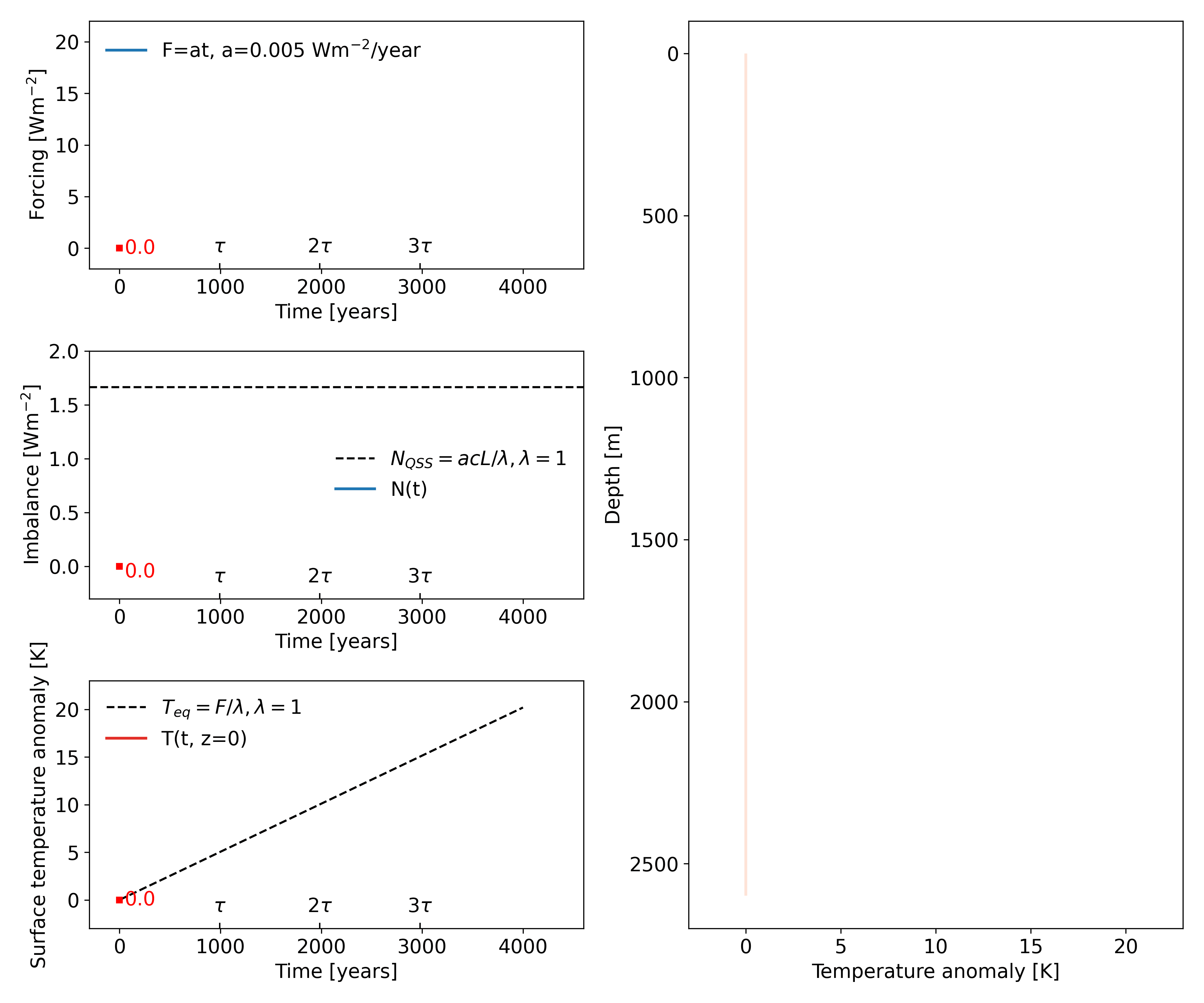
The climate feedback parameter \(\lambda [\mathrm{Wm}^{-2} \mathrm{K}^{-1}]\) is comprised of a change in the Plank emissivity, increased water vapour content, etc. It is assumed constant and the temperature response to forcing is assumed linear for the small ranges of interest. An Earth’s atmosphere representative value is \(\lambda = 1 \mathrm{Wm}^{-2}\mathrm{K}^{-1}\). A doubling of carbon dioxide concentrations amounts to a forcing of around \(F = 4 \mathrm{Wm}^{-2}\).

To gain intuition for the temperature change over time, the effective heat capacity of the system needs to be accounted for. A simple model for this is a one-dimensional diffusive domain, in which the heat conductivity coefficient accounts for the ocean processes which mix the warmed waters in the upper layers with those below. To treat the problem analytically, we assume that mixing is proportional to the temperature difference and the heat conductivity parameter \(K [\mathrm{Wm}^{-1}\mathrm{K}^{-1}]\) is assumed constant in depth. An Earth’s oceans representative value is \(K = 350 \mathrm{Wm}^{-1}\mathrm{K}^{-1}\) with a heat capacity of seawater of \(c = 4 \times 10^6 \mathrm{Jm}^{-3}\mathrm{K}^{-1}\).

Setting the 1D heat equation with upper Robin and lower Neumann boundary conditions describes the forcing-feedback energy input at the top and ensures energy conservation by no flux leakage at the bottom.

For linearly increasing forcing \(F = at\), the system has a quasi-steady state solution in which the temperature tendency is constant and so is the energy imbalance. The timescale \(\tau\) to approach this quasi-steady state is a property of the system (i.e. a function of \(c, K, L\)), and is independent of the forcing rate \(a\) or total forcing \(at\). Inserting numerical values (\(L=2600\)m, \(K=350\)Wm\(^{-1}\)K\(^{-1}\), \(c=4\times10^6\)Jm\(^{-3}\)K\(^{-1}\)), we obtain \(\tau \approx 990\)years.

The take-home from solving this problem analytically is that for a linear system with linear forcing, we expect the energy imbalance to grow and the surface temperature to accelerate even after \(\sim 100\) years of linear forcing. This is because the timescale to approach quasi-steady state is \(\sim 1000\) years.

A press-release for this article has been posted within the Wolfram Community.